Gathering Intel on Intel AVX-512 Transitions
Introduction
This is a post about AVX and AVX-512 related frequency scaling1.
Now, something more than nothing has been written about this already, including cautionary tales of performance loss and some broad guidelines2, so do we really need to add to the pile?
Perhaps not, but I’m doing it anyway. My angle is a lower level look, almost microscopic really, at the specific transition behaviors. One would hope that this will lead to specific, quantitative advice about exactly when various instruction types are likely to pay off, but (spoiler) I didn’t make it there in this post.
Now I wasn’t really planning on writing about this just now, but I got off on a (nested) tangent3, so let’s examine the AVX-512 downclocking behavior using target tests. At a minimum, this is necessary background for the next post, but I hope that it is also standalone interesting.
Note: For the really short version, you can skip to the summary, but then what will do you for the rest of the day?
Table of Contents
You could perhaps trying skipping ahead to a section that interests you using this obligatory table of contents, but sections are not self contained, so you’ll be better off reading the whole thing linearly.
The Source
All of the code underlying this post is available in the post1 branch of freq-bench, so you can follow along at home, check my work, and check out the behavior on your own hardware. It requires Linux and the README gives basic clues on getting started.
The source includes the data generation scripts as well as those to generate the plots. Neither shell scripting nor Python are my forte, so be gentle.
Test Structure
We want to investigate what happens when instruction stream related performance transitions occur. The most famous example is what happens when you execute an AVX-512 instruction4 for the first time in a while, but as we will see there are other cases.
The basic idea is that the test has a duty period and every time this period elapses, we run a test-specific payload for the duration of the payload period which consists of one or more “interesting” instructions (which depend on the test). During the entire test we sample various metrics at a best-effort fixed frequency. This repeats for the entire test period. The sample period will generally be much smaller than the duty period5: in our tests we use a 5,000 μs duty period and a sample period of 1 μs, mostly.
Visually, it is something like this (showing a single duty period: one benchmark is composed of multiple duty cycles back to back):
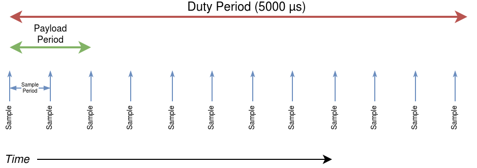
This diagram shows the payload period as occupying a non-negligible amount of time. However, in the first few first tests, the payload period is essentially zero: we run the payload function (which consists of only a couple instructions) only once, so it is really a payload moment rather than period.
Hardware
We are running these tests on a SKX architecture W-series CPU: a W-21046 with the following license-based frequencies7:
| Name | License | Frequency |
|---|---|---|
| Non-AVX Turbo | L0 | 3.2 GHz |
| AVX Turbo | L1 | 2.8 GHz |
| AVX-512 Turbo | L2 | 2.4 GHz |
For one (voltage) test I also use my Skylake (mobile) i7-6700HQ, running at either it’s nominal frequency of 2.6 GHz, or the turbo frequency of 3.5 GHz.
Tests
The basic approach this post will take is examining the CPU behavior using the test framework above, primarily varying what the payload is, and what metrics we look at. Let’s get the ball rolling with 256-bit instructions.
256-bit Integer SIMD (AVX)
For the first test will use as payload the vporymm_vz function, which is just a single 256-bit vpor instruction, followed by a vzeroupper8:
vporymm_vz:
  vpor   ymm0,ymm0,ymm0
  vzeroupper
  ret
We call the payload function only once at the start of each duty period9. The duty period is set to 5000 μs and the sample period to 1 μs, and the total test time is set to 31,000 μs (so the payload will execute 7 times).
Here’s the result (plot notes10), with time along the x axis11, showing the measured frequency at each sample (there are three separate test runs shown12):
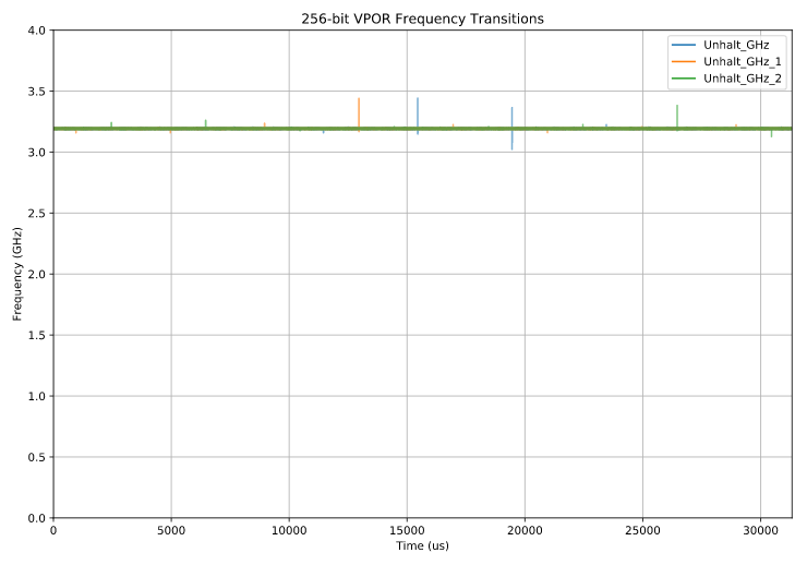
Well that’s really boring. The entire test runs consistently at 3.2 GHz, the nominal (L0 license) frequency, if we ignore the a few uninteresting outliers13.
512-bit Integer SIMD (AVX-512)
Before the crowd gets too rowdy, let’s quickly move on to the next test, which is identical except that it uses 512-bit zmm registers:
vporzmm_vz:
  vpor   zmm0,zmm0,zmm0
  vzeroupper
  ret
Here is the result:
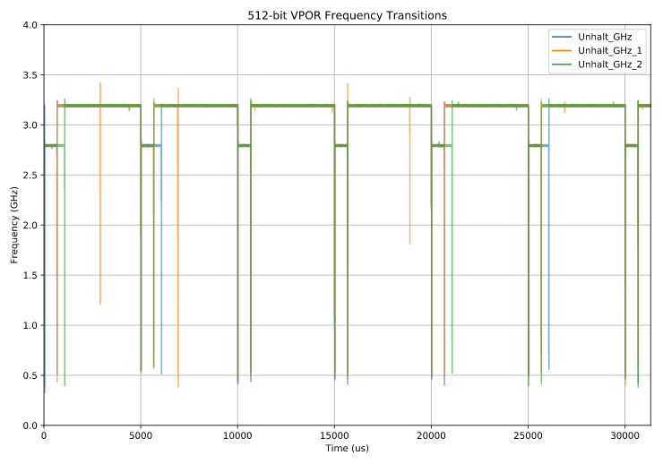
We’ve got something to sink our teeth into!
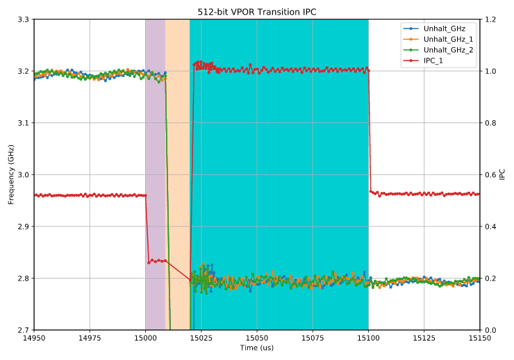
Remember that the duty cycle is 5000 μs, so at each x-axis tick we execute the payload. Now the behavior is clear: every time the payload instruction executes (at multiples of 5000 μs), the frequency drops from the 3.2 GHz L0 license down to 2.8 GHz L1 license frequency. So far this is all pretty much as expected.
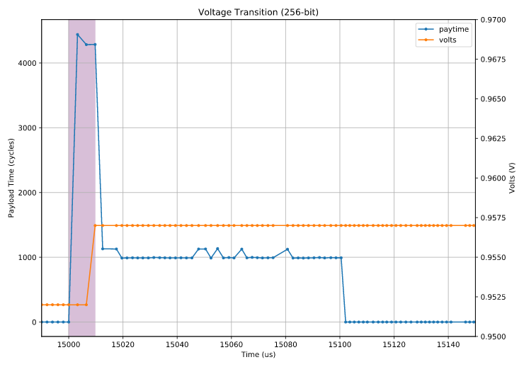
Let’s zoom in on one of the transition points at 15,000 μs:
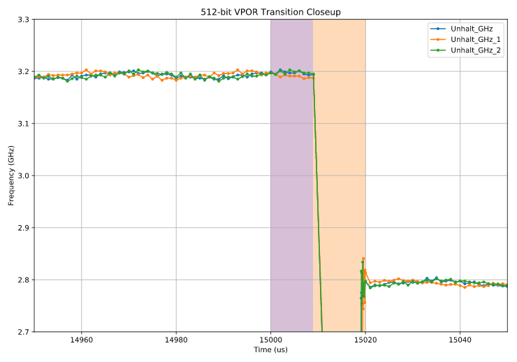
We can make the following observations:
- There is a transition period (the rightmost of the two shaded regions, in orange14) of ~11 μs15 where the CPU is halted: no samples occur during this period16. For fun, I’ll call this a frequency transition.
- The leftmost shaded region, shown in purple17, immediately following the payload execution at 15,000 μs and prior to the halted region, is ~9 μs long and the frequency remains unchanged. This is not just a test issue or measurement error: this period occurs after the payload and is consistently reproducible18. Although it looks like nothing interesting is going on in this region, we’ll soon see it is indeed special and will call this region a voltage-only transition.
- Although not fully shown in the zoomed plot, the lower 2.8 GHz frequency period lasts for ~650 μs.
- Not shown in the zoomed plot (but seen as a second downwards spike on the full plot, after the ~650 μs period of low frequency), there is another fully halted period of ~11 us, after which the CPU returns to it’s maximum speed of 3.2 GHz (L0 license).
- These attributes are mostly consistent across the three runs (so much that the series, in green, mostly overlaps and obscures the others) – but there are a few outliers in where the return to 3.2 GHz takes somewhat longer. This is consistent across runs: recovery is never faster than ~650 μs, but sometimes longer. I believe it occurs when an interrupt during the L1 region “resets the timer”.
Enter IPC
Although it is not visible in this plot, there is something special about the behavior of 512-bit instructions in the first shaded (purple) region – that is, in the 9 microseconds between the execution of the payload instruction and before the subsequent halted period: they execute much slower than usual.
This is easiest to see if we extend the payload period: instead executing the payload function once every 5000 μs, then looping on rdtsc, waiting for the next sample, we will continue to execute the payload function for 100 μs after a new duty period starts (that is, the payload period is set to 100 μs). During this time we still take samples as usual, every 1 μs – but in between samples we are executing the payload instruction(s)19. So one duty period now looks like 100 μs of payload followed by 4850 μs of normal payload-free hot spinning.
We lengthen the payload period in order to examine the performance of the payload instructions. There are several metrics we could look at, but a simple one is to look at instructions per second. As long as we make sure the large majority of the executed instructions are payload instructions, the IPC will largely reflect the execution of the payload20.
As payload, we will use a function composed simply of 1,000 dependent 512-bit vpord instructions:
vpord  zmm0,zmm0,zmm0
vpord  zmm0,zmm0,zmm0
; ... 997 more like this
vpord  zmm0,zmm0,zmm0
vzeroupper
ret
We know these vpord instructions have a latency of 1 cycle and here they are serially dependent so we expect this function to take 1,000 cycles, give or take21, for an IPC of 1.0.
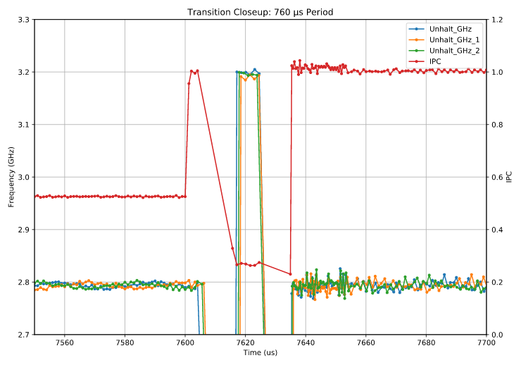
Here’s what a the same zoomed transition point for this looks like, with IPC plotted on the secondary axis:
First, note that in the unshaded regions on the left (before 15,000 μs) and right (after 15,100 μs), the IPC is basically irrelevant: no payload instructions are being executed, so the IPC there is just the whatever the measurement code happens to net out to. We only care about the IPC in the shaded regions, where the payload is executing.
Let’s tackle the regions from right to left, which happens to correspond to obvious to less obvious.
We have the blue region, running from ~15020 μs to 15100 μs (where the extra payload period ends). Here the IPC is right at 1 instruction per cycle. So the payload is executing right at the expected rate, i.e., full speed. Keeners may point out that the very beginning of the blue period, the IPC (and the measured frequency) is a bit noisier and slightly above 1. This is not a CPU effect, but rather a measurement one: during this phase the benchmark is catching up on samples missed during the previous halted period, which changes the payload to overhead ratio and bumps up the IPC (details22).
The middle, orange, region shows us what we’ve already seen: the CPU is halted, so no samples occur. IPC doesn’t tell us much here.
Voltage Only Transitions
The most interesting part is the first shaded region (purple): after the payload starts running but before the halt which I call a voltage only transition for reasons that will soon become clear.
Here, we see that the payload executes much more slowly, with an IPC of ~0.25. So in this region, the vpord instructions are apparently executing at four times their normal latency. I also observe an identical 4x slowdown for vpord throughput, using an identical test except with independent vpord instructions23.
Perhaps surprisingly, this same slowdown occurs for 256-bit ymm instructions as well. This contradicts the conventional wisdom that on AVX-512 chips there is no penalty to using light 256-bit instructions:
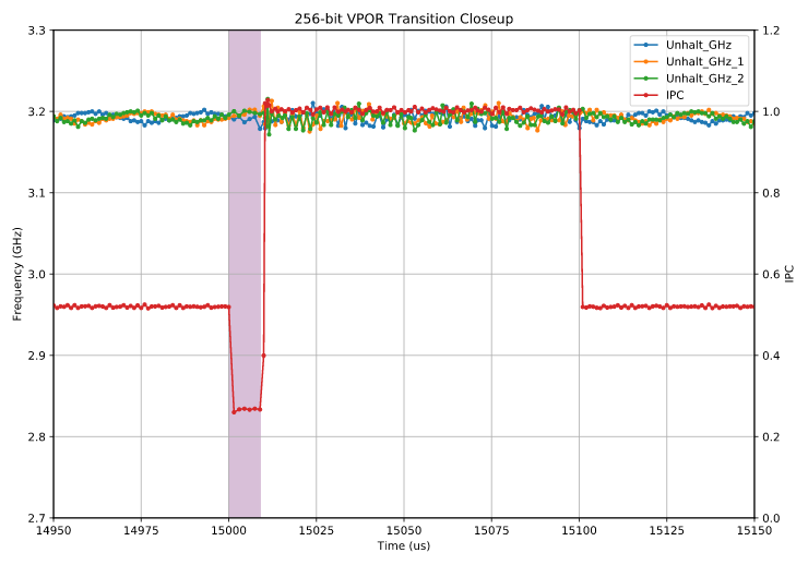
The results shown above are for a test identical to the 512-version except that it uses 256-bit vpor ymm0, ymm0, ymm0 as the payload. It shows the same slowdown for ~9 μs after the payload starts executing, but no subsequent halt and no frequency transition. That is, it shows a voltage-only transition (lack of frequency transition is expected because we don’t expect a turbo license change for light 256-bit instructions).
By now, you are probably wondering about 128-bit xmm registers. The good news is that these show no effect at all:
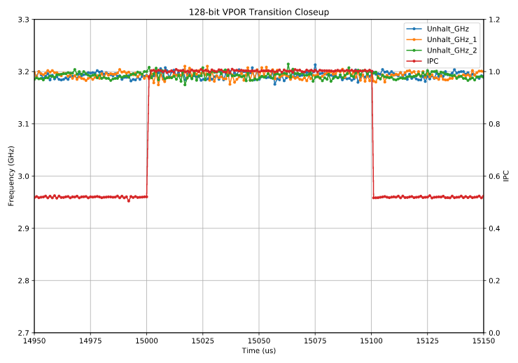
Here, the IPC jumps immediately to the expected value. So it appears that the CPU runs in a state where the 128-bit lanes are ready to go at all times24.
The conventional wisdom regarding this “warmup” period is that the upper part25 of the vector units is shut down when not in use, and takes time to power up. The story goes that during this power-up period the CPU does not need to halt but it runs SIMD instructions at a reduced throughput by splitting up the input into 128-bit chunks and passing the data two or more times through the powered-on 128-bit lanes26.
However, there are some observations that seem to contradict this hypothesis (in rough order from least to most convincing):
- The observed impact to latency and throughput is ~4x, whereas I would expect 2x for simple instructions such as
vpor. - The timing is the same for 256-bit and 512-bit instructions: despite that 512-bit instructions take at least 2x the work, i.e., need to be passed through the 128-bit unit at least 4 times.
- Some instructions are more difficult to implement using this type of splitting, e.g., instructions where both high and low output lanes depend on all of the input lanes27 (see how slow they are on Zen). I expected that maybe these instructions would be slower when running in split mode, but I tested
vpermdand found that it runs at 4L4T28, compared to 3L1T normally. Sovpermd(including the 512-bit version) didn’t slow more thanvpor, and in fact in a relative sense it slowed down less (e.g., the latency only changed from 3 to 4). The fact that the latency and throughput reacted differently for this instruction seems odd, and that it has now the exact same 4L4T timing asvporseems like a strange coincidence. - Oddly, when I tried to time the slowdown more precisely, I kept coming with fractional value around 4.2x, not 4.0x, kind of contradicting the idea that the instruction is simply operating in a different mode, which should still have an integral latency.
- As it turns out, all ALU29 instructions are slower in this mode, not just wide SIMD ones.
It was 5 that sealed the deal on this not being a slowdown related to split execution. I believe what is actually happening is the CPU is doing very fine-grained throttling when wider instructions are executing in the core. That is, the upper lanes are being used in this mode (they are either not gated at at all, or are gated but enabling them is very quick, less than 1 μs) but execution frequency is reduced by 4x because CPU power delivery is not a state that can handle full-speed execution of these wider instructions, yet. While the CPU waits (e.g., for voltage to rise, fattening the guardband) for higher power execution to be allowed, this fine-grained throttling occurs.
This throttling affects non-SIMD instructions too, causing them to execute at 4x their normal latency and inverse throughput. We can show with the following test, which combines a single vpor ymm0, ymm0, ymm0 with N chained add eax, 0 instructions, shown here for N = 3:
vpor   ymm0,ymm0,ymm0
add    eax,0x0
add    eax,0x0
add    eax,0x0
; repeated 9 more times
If only vpor is slowed down, each block of 4 instructions will take 4 cycles, limited by the vpor chain (the add chain is 3 cycles long). However, I actually measure ~12 cycles, indicating that we are instead limited by the add chain, each of which takes 4 cycles for a total of 12.
We can vary the number of add instructions (N) to see how long this effect persists. This table is the result:
| ADD instructions (N) | Cycles/ADD | Delta Cycles (slow) | Delta Cycles (fast) |
|---|---|---|---|
| 2 | 4.1 | 2.3 | -0.2 |
| 3 | 4.1 | 4.0 | 0.8 |
| 4 | 4.1 | 4.1 | 1.1 |
| 5 | 4.0 | 3.9 | 1.1 |
| 6 | 4.1 | 4.3 | 0.7 |
| 7 | 4.0 | 3.4 | 1.1 |
| 8 | 4.0 | 4.2 | 0.9 |
| 9 | 4.1 | 3.9 | 0.8 |
| 10 | 4.1 | 4.3 | 1.1 |
| 20 | 4.0 | 4.0 | 1.0 |
| 30 | 4.0 | 4.0 | 1.0 |
| 40 | 4.1 | 4.3 | 1.0 |
| 50 | 4.1 | 3.9 | 1.0 |
| 60 | 4.1 | 4.4 | 1.0 |
| 70 | 4.2 | 4.5 | 1.0 |
| 80 | 4.1 | 3.4 | 1.0 |
| 90 | 3.6 | -0.2 | 1.0 |
| 100 | 3.3 | 1.1 | 1.0 |
| 120 | 2.9 | 0.9 | 1.0 |
| 140 | 2.7 | 1.1 | 1.0 |
| 160 | 2.5 | 1.2 | 1.0 |
| 180 | 2.3 | 0.7 | 0.9 |
| 200 | 2.2 | 0.8 | 1.0 |
The Cycles/ADD column shows the number of cycles taken per add instruction over the entire slow region (roughly the first 8-10 μs after the payload starts executing). The Delta Cycles (slow) shows how many cycles each additional add instruction took compared to the previous row: i.e., for row N = 30, it determines how much longer the 10 additional add instructions took compared to the row N = 20. The Delta Cycles (fast) column is the same thing, but applies to the samples after ~10 μs when the CPU is back up to full speed (that column shows the expected 1.0 cycles per additional add).
Here we clearly see that up to roughly 70 add instructions, interleaved with a single vpor, all the add instructions are taking 4 cycles, i.e., the CPU is throttled. Somewhere between 80 and 90 a transition happens: additional add instructions now take 1 cycle, but the overall time per add is (initially) close to 4. This shows that when add (and presumably any non-wide instruction) is far enough away from the closest wide SIMD instruction, they start executing at full speed. So the timings for the larger N values can be understood as a blend of a slow section of ~70-80 add instructions near the vpor which run at 1 per 4 cycles, and the remaining section where they run at full speed: 1 per cycle.
We can probably conclude the CPU is not just throttling frequency or “duty cycling”: in that case every instruction would be slowed down by the same factor, but instead the rule is more like “latency extended to the next multiple of 4 cycles”, e.g., a latency 3 instruction like imul eax, eax, 0 ends up taking 4 cycles when the CPU is throttling. It is likely that the throttling happens at some part of the pipeline before execution, e.g., at issue or dispatch.
The transition to fast mode when the vpor instructions are spread sufficiently apart probably reflects the size of some structure such as the IDQ (64 entries in Skylake) or scheduler (97 entries claimed30). The core could track whether any wide instruction currently in that structure, and enforce the slow mode if so. The vpor instructions are close enough together, there is always at least one present, but once they are spaced out enough, you get periods of fast mode.
Voltage Effects
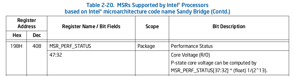
We can actually test the theory that this transition is associated with waiting for a change in power delivery configuration. Specifically, we can observe the CPU core voltage, using bits 47:32 of the MSR_PERF_STATUS MSR. Volume 4 of the Intel Software Development Manual let’s us on a secret: these bits expose the core voltage31:
Let’s zoom as usual on a transition point, in this case using a 256-bit (ymm) payload of 1000 dependent vpor instructions. This 256-bit payload means no frequency transition, only a dispatch throttling period associated with running 256-bit instructions for the first time in a while. We plot the time it takes to run an iteration of the payload32, along with the measured voltage:
The length of the throttling period is around 10 μs as usual, as shown by the period where the payload takes ~4,000 cycles (the usual 4x throttling), and the voltage is unchanged from the pre-transition period (at about 0.951 V) during the throttling period. At the moment the throttling stops, the voltage jumps to about 0.957, a change of about 6 mV. This happens at 2.6 GHz, the nominal non-turbo speed of my i7-6700HQ. At 3.5 GHz, the transition is from 1.167 to 1.182, so both the absolute voltages and the difference (about 15 mV) are larger, consistent the basic idea that higher frequencies need higher voltages.
So one theory is that this type of transition represents the period between when the CPU has requested a higher voltage (because wider 256-bit instructions imply a larger worst-case current delta event, hence a worst-case voltage drop) and when the higher voltage is delivered. While the core waits for the change to take effect, throttling is in effect in order to reduce the worst-case drop: without throttling33 there is no guarantee that a burst of wide SIMD instructions won’t drop the voltage below the minimum voltage required for safe operation at this frequency.
Attenuation
We might check if there is any attenuation of either type of transition. By attenuation I mean that if a core is transitioning between frequencies too frequently, the power management algorithm may decide to simply keep the core at the lower frequency, which can provide more overall performance when considering the halted periods needed in each transition. This is exactly what happens for active core count34 transitions: too many transitions in a short period of time and the CPU will just decide to run at the lower frequency rather than incurring the halts need to transition between e.g. the 1-core and 2-core turbos35.
We check this by setting a duty period which is just above the observed recovery time from 2.8 to 3.2 GHz, to see if we still see transitions. Here’s a duty cycle of 760 μs, about 10 μs more than the observed recovery period for this test36:
I’m not going to color the regions here, as by now I think you are probably (over?) familiar with them. The key points are:
- The payload starts executing at 7600 μs, which is before the upwards frequency transition, we are still executing at 2.8 GHz - so initially the IPC is high, 1 per cycle.
- Despite the fact that we are already executing again 512-bit instructions, the frequency adjusts upwards a few μs later. Most likely what happened is that the power logic already evaluated earlier (say at ~7558 μs, just before the payload started) that an upwards transition should occur, but as we’ve seen the response is generally delayed by 8 to 10 μs so it occurs after the payload has already started executing.
- Of course, as soon as the transition occurs, the core is no longer in a suitable state for full-speed wide SIMD execution, so IPC drops to ~0.25.
- Another transition back to low frequency occurs ~10 μs later and then full speed execution can resume.
So there is no attenuation, but attenuation isn’t really needed: the long (~650 μs) cooldown period between the last wide instruction and subsequent frequency boost means that the damage from halt periods are fairly limited: this is unlike the active core count scenario where the CPU has no control over the transition frequency (rather it is driven by interrupts and changes in runnable processes and threads). Here, we have the worst case scenario of transitions packed as closely as possible, but we lose only ~20 μs (for 2 transitions) out of 760 μs, less than a 3% impact. The impact of running at the lower frequency is much higher: 2.8 vs 3.2 GHz: a 12.5% impact in the case that the lowered frequency was not useful (i.e., because the wide SIMD payload represents a vanishingly small part of the total work).
What Was Left Out
There’s lots we’ve left out. We haven’t even touched:
- Checking whether xmm registers also cause a voltage-only transition, if they haven’t been used for a while. We didn’t find any effect, but it also certain that some 128-bit instructions appear in the measurement loop which would hide the effect.
- Checking whether the voltage-only transition implied by 256-bit instructions are disjoint from those for 512-bit. That is, if you execute a 256-bit instruction after a while without any, you get a voltage-only transition (confirmed above). If you then execute a 512-bit instruction, before the relaxation period expires, do you get a second throttling period prior to the frequency transition? I believe so but I haven’t checked it.
- Any type of investigation of “heavy” 256-bit or 512-bit instructions. These require a license one level (numerically) higher than light instructions, and knowing if any of the key timings change would be interesting37.
- Almost no investigation was made how any of these timings (and the magnitude of voltage changes) vary with frequency. For example, if we are already running at a lower frequency, frequency transitions are presumably not needed, and voltage-only transitions may be shorter.
Summary
For the benefit of anyone who just skipped to the bottom, or whose eyes glazed over at some point, here’s a summary of the key findings:
- After a period of about 680 μs not using the AVX upper bits (255:128) or AVX-512 upper bits (511:256) the processor enters a mode where using those bits again requires at least a voltage transition, and sometimes a frequency transition.
- The processor continues executing instructions during a voltage transition, but at a greatly reduced speed: 1/4th the usual instruction dispatch rate. However, this throttling is fine-grained: it only applies when wide instructions are in flight (details).
- Voltage transitions end when the voltage reaches the desired level, this depends on the magnitude of the transition but 8 to 20 μs is common on the hardware I tested.
- In some cases a frequency transitions is also required, e.g., because the involved instruction requires a higher power license. These transitions seem to first incur a throttling period similar to a voltage-only transition, and then a halted period of 8 to 10 μs while the frequency changes.
- A key motivator for this post was to give concrete, qualitative guidance on how to write code that is as fast as possible given this behavior. It got bumped to part 2.
We also summarize the key timings in this beautifully rendered table:
| What | Time | Description | Details |
|---|---|---|---|
| Voltage Transition | ~8 to 20 μs | Time required for a voltage transition, depends on frequency | 38 |
| Frequency Transition | ~10 μs | Time required for the halted part of a frequency transition | 39 |
| Relaxation Period | ~680 μs | Time required to go back to a lower power license, measured from the last instruction requiring the higher license | 40 |
Thanks
Daniel Lemire who provided access to the AVX-512 system I used for testing.
David Kanter of RWT for a fruitful discussion on power and voltage management in modern chips.
RWT forum members anon³, Ray, Etienne, Ricardo B, Foyle and Tim McCaffrey who provided feedback on this post and helped me understand the VR landscape for recent Intel chips.
Alexander Monakov, Kharzette and Justin Lebar for finding typos.
Jeff Smith for teaching me about spread spectrum clocking.
Discuss
Discussion on Hacker News, Twitter and lobste.rs.
Direct feedback also welcomed by email or as a GitHub issue.
If you liked this post, check out the homepage for others you might enjoy.
-
… and also non frequency related performance events, which I mention only in a footnote not to spoil the fun for non-footnote type people and also to pad by footnote count. That’s why I call this Performance Transitions, instead of Frequency Transitions. ↩
-
Note that Daniel has written much more than just that one. ↩
-
This was going to be the actual post I was trying to write when I went off on this tangent about clang-format. In fact I was writing that post, when I went off this current tangent, but then a footnote turned into several paragraphs, then got its own section and ultimately graduated into a whole post: the one you are reading. So consider this background reading for the “interesting” post still to come, although honestly the stuff here is probably more generally useful than the next part. ↩
-
We should be clear here: when I say AVX-512 instruction in this context, I mean specifically a 512-bit wide instruction (which currently only exist in AVX-512). The distinction is that AVX-512 includes 128-bit and 256-bit versions of almost every instruction it introduces, yet these narrower instructions behave just like 128-bit SSE* and 256-bit AVX* instructions in terms of performance transitions. So, for example,
vpermwis unabiguously AVX-512 instruction: it only exists in AVX-512BW, but only the version that takeszmmregisters causes “AVX-512 like” performance transitions: the versions that takeymmorxmmregisters act as any other integer 256-bit AVX2 or 128-bit SSE instruction. ↩ -
In fact, we generally want the sample period to be as small as possible, to give the best resolution and insight into short-lived events. We can’t make it too short though as the samples themselves have a minimum time to capture, and very short samples tend to be noisy due to non-atomicity, quantization effects, etc. ↩
-
The CPU is an Intel W-2104, a Xeon-W chip based on the SKX uarch. It has no turbo and an on-the-box speed of 3200 MHz, but accurate tools will probably report it running at 3192 MHz due to spread spectrum clocking (SSC). In fact, we can see the typical 0.5% spread spectrum triangle wave on almost any of the plots in this post, at the right zoom level, like this one. This occurs because we measure time (the x-axis) based on
rdtscwhich is based off of a different clock not subject to SSC, while the unhalted cycles counter counts CPU cycles, which are based off of the 100 MHz BLCK which is subject to SSC. ↩ -
This is the part where I just gloss over what that
vzeroupperis doing there. It’s there due to implicit widening. That’s a new term I just invented and it’s the first and last time I’m mentioning it this post, because it really deserves an entire post of its own. The very short version is that any time an SIMD instruction writes to an N-bit register (N in {256, 512}), all subsequent SIMD instructions are implicitly N bits wide, regardless of their actual width, for the purposes of determining turbo licenses and other transitions discussed here. This sounds a bit like the mixed-VEX penalties thing, but it is very different. This a mini-bombshell hidden in a footnote, so if you want to scoop me you can, but I’m not coming to your birthday party. ↩ -
I.e., the payload period is zero, but the structure of the test ensures the function is called once, at the start of the payload period, no matter how small the payload period is. ↩
-
All of the plots in this post are SVG images, meaning they can be zoomed arbitrarily: so if you want to zoom in on any region feel free (the browser limits the zoom amount, but just save as a file and open it with any SVG viewer). ↩
-
These are basically a poor man’s version of the Falk Diagrams that Brandon Falk describes in this post among others. Poor in the sense that they have ~3000 cycle resolution instead of 1 cycle resolution, and because the measurement code has to be integrated directly into the system under test. Basically they are nothing like Falk Diagrams except that they have time on the x-axis and some performance counter event on the y-axis, but they are good enough for our purposes. ↩
-
Specifically, all three runs are identical and I show them just to give a rough impression of which effects are reproducible and which are outliers. The second and third runs have the suffixes
_1and_2, respectively, in the legends. ↩ -
These outliers usually occur when an interrupt occurs during the measurement. Originally I used a 3 μs sample time, and there were almost no visible outliers with that period, but the 1 μs value I settled on is much better in most respects other than outliers. The main problem is when an interrupt takes more than the sample time of ~1 μs: this causes one or more samples to be very short, because a long sample will cause subsequent ones to be short (maybe very short) until we catch up to the fixed sample schedule, and very short samples are subject to much more noise because the absolute metric values are much smaller but the error sources usually have fixed absolute error. Another source of outliers is when an interrupt splits the stamp: the stamp is the series of metrics we calculate at the sample point. These various metrics aren’t sampled atomically: if an interrupt occurs in the middle of the sampling, some metrics will reflect a much shorter time period (before the interrupt) and some a longer one (after). This effect tends to cause bidirectional spike outliers: where an upspike and downspike occur in consecutive samples. I try to avoid this by retrying the stamp if I think I’ve detected an interrupt during measurement (up to a retry limit). We could avoid all this nonsense by running the benchmark itself in the kernel, where we can disable interrupts (although some SMIs might still sneak in). Maybe next time! ↩
-
Note that the resolution of the sampling is 1 μs, so when we say things like 9 μs and 11 μs it could be off by up to 1 μs. This 1 μs “error” isn’t exactly randomly distributed, because the sampling interval is “exact” and in phase with the payload execution. So the samples are always at 1.0, 2.0, 3.0, … μs after the payload executes (plus or minus small variation on the order of 10 nanoseconds), so if the true time until halt is anywhere between 9.00 and 9.99 μs, we will always read 9 μs (because time shown for the sample is the end of the sample and covers the preceding 1 us). For the halt time, the scenario is reversed: the start of the interval is uncertain, but the end should be exact modulo the delay in taking the sample. ↩
-
Generally you can detect halted periods when
rdtscjumps forward, but performance counters like “non-halted cycles” do not, and there are not indications of a larger interruption such as a context switch. You can find a similar case of halted periods in this question which was also caused by frequency transitions (in this case, to obey the different active core count turbo ratios). ↩ -
In particular, I have confirmed that these three samples all occur after the payload has executed and retired using the period column in the output, which indicates clearly which sames are before or after a given execution of the payload. The payload itself is followed by an
lfenceto ensure it has retired before taking further samples (and in any case the number of instructions per sample is too large be accommodated by the OoO window). ↩ -
Those who are still awake at this point might be wondering why introduce this new variant of the test now: why not just execute the payload instructions during the wait period in the original tests too? One reason is that by hot spinning on
rdtscwe get somewhat more consistent results when we care only about measuring the frequency in that we almost always sample at exactly the specified period (plus or minus therdtsclatency, more or less). When we execute the longish payload function during the wait, the sample point diverges a bit more from the ideal, and the number of spins per sample suffers more quantization effects (i.e., the pattern of spin counts might be 3,3,3,2,3,3,3,2… rather than 450,450,451,450…), which can sometimes lead to a slight sawtooth effect in the samples. ↩ -
In practice, we don’t exactly reach this ideal: we execute the payload function 2 or 3 times, for 2,000 or 3,000
vporinstructions, but there are about 600 additional instructions of overhead associated with taking a sample, so the overhead instructions are a significant portion. Probably 600 instructions is too many, I haven’t optimized that and it could likely be lowered significantly. However, we can also improve the ratio simply by decreasing the sampling resolution (i.e., increasing the sampling time). I selected 1 μs as a tradeoff between these competing factors. Note: Since I wrote this footnote I optimized several things in the sampling loop, so measured IPCs are now very close to their theoretical values, but I guess this footnote still has value?. ↩ -
The main uncertainty in the timing of the function itself concerns the boundary conditions: if we run this function 10 times without touching
zmm0in between, the dependency onzmm0will be carried between functions and the total time will be very close to 10 x 1000 = 10,000 cycles. However, if some compiler generated code in between calls to the payload function happens to write tozmm0, breaking the dependency, the individual chains for each function no longer depend on each other, so some overlap is possible. The amount of this overlap is limited by the size of the RS, so the effect won’t be huge but it could be noticeable (with say 100 payload instructions rather than 1,000 it could be very significant). We basically sidestep this whole issue by putting anlfencebetween each call to the payload function, which forms an execution barrier between calls. ↩ -
The way the sampling works in this test could be described locked interval without skipping. Here, locked interval means we calculate the next target sample time based on the previous target sample time (rather than the actual sample time), plus the period. So if we are sampling at 10 μs, the target sample times will always be 10 μs, 20 μs, etc. In particular, the series of target sample time doesn’t depend on what happens during the test, e.g., it doesn’t depend on the actual sample time: even if we actually end up sampling at time = 12 μs rather than 10, we target time = 20 μs as the next sample, not 12 + 10 = 22 μs. This raises the question about what happens when some delay (e.g., an interrupt, a frequency transition) causes us to miss more than 1 entire sample period.
E.g., with 10 μs resolution we just sampled at 90 μs, so the next sample target is 100 μs, but a delay causes the next sample to be taken at 125 μs. We are now behind! The next sample should occur at 110 μs, but of course that is in the past. The current test design still takes all the required samples, as quickly as possible (but with a minimum of one payload call if we are in the extra payload period) – that’s the no skipping part. In the current example, it means we would take subsequent samples quickly until we are caught up, at say 125 μs (target 110 μs), 126 μs (target 120 μs), 130 μs (target 130 μs), with that last sample being “on target”.
These samples occur quickly: very quickly in the case of normal samples which take less than 0.2 μs each, or more slowly in the case of the extra payload region, where the payload call bumps that to about 0.5 μs. So that’s what’s happening in the green region: we just had a frequency transition halt of ~10 μs, so we are ~10 samples beyind and so the following samples are taken more quickly (as you can see because the data point markers are spaced more closely), with only a single payload call each (versus 2 or 3 usually). This changes the ratio of payload instructions to overhead instructions, which tends to bump the IPC a bit (for the same reason the caught-up blue region almost shows IPC > 1). This effect can be reduced or eliminated by increasing the sampling period, since that reduces the number of catchup samples.
Incidentally, this also explains the oscillating pattern you see in the blue region: the ideal number of payload calls to get a 1 μs sample rate is ~2.5, so the sampling strategy tends to alternative between two and three calls: more calls means IPC closer to 1: so the peaks of the oscillating are two calls and the valleys, three. ↩
-
I’m not going to fully analyze the throughput case, but the thorough among us can find the chart here. Note that the overhead here cuts the other way: pushing the IPC below the expected value of 2.0 (there are 2 512-bit vector units capable of executing
vpord) because here the throughput limited instructions compete for ports with the overhead instructions. ↩ -
Of course, another possibility is that something in the rest of the test loop uses
xmmregisters so they remain “hot”: they are “baseline” for x86-64 after all, so the compiler is free to use them without any special flags. We could test this theory with a more compact test loop audited to be free of anyxmmuse… but I’m not going to bother. I’m pretty sure these guys are powered up all the time as their use is pervasive in most x86-64 code. ↩ -
Specifically, the the part handing the second (bits 128:255) for the
ymmcase, and the upper 3 lanes (bits 128:511) in thezmmcase. ↩ -
This isn’t far fetched - that’s exactly how AMD Zen always executes 256-bit AVX instructions with its 128 bit units, and similar to how SVB and IVB did the same for 256-bit load and store instructions. So using narrower vector units to implement wider instructions is definitely a thing. ↩
-
These are usually called cross lane instructions (where a lane is 128 bits on Intel). For example,
vporis not like this: it is an element-wise operation where each output element (down to each bit, in this case) depends only on the element in the same position in the input vectors. On other the hand,vpermdis: each 32-bit element in the output can come from any position in the input vector (but it still behaves as element-wise wrt the mask register41). ↩ -
The notation 4L4T means: “4 cycles of latency and 4 cycles of inverse throughput”. That is, an given instance of this instruction takes 4 cycles to finish (latency), and a new instruction can start every 4 cycles (inverse throughput, hence the throughput is 0.25). When the CPU is running normally, most single-uop SIMD instructions have latency of 1 (in lane), 3 (most cross lane integer or shuffle ops) or 4 (most FP arithmetic). ↩
-
I say ALU instructions here, but I strongly suspect it might be all instructions: you can certainly test that at home using the same test (the
vporxymm250_*group of tests) but with other types of instructions such as loads replacing theadd. I didn’t really test all ALU instructions either: just a few - but it is fair to assume that ifaddis slowed down, it is something generic, probably affecting at least all ALU stuff, not something instruction specific. ↩ -
Documentation claims 97 entries, but my testing seems to indicate they are not unified in Skylake: apparently only 64 can be used for ALU ops, and 33 for memory ops. ↩
-
Try as I might, I can’t determine if this refers to measured core voltage, i.e., true voltage as determine at some sensor within the core, or demanded voltage, i.e., the voltage the processor wants right now based on the various power-relevant parameters, sometimes called the VID. In any case, we expect those values to track each other fairly closely, perhaps with some offset and since we are looking for voltage changes either one works. That said, I am very interested if you know the answer to this question. ↩
-
This payload time series is meant to show the exact same thing as the IPC series in earlier charts: we just want an indication of when the Type 1 throttling starts and stops. I used IPC initially because it was easy (I didn’t have to instrument the payload section specially) - but it doesn’t work when reading volts because that measurement involves a ton of additional instructions and a user-kernel transition, so it throws the IPC off completely. So I went ahead and instrumented the payload section directly, so we can still see the throttling, but no way I want to go back and change the other plots that use IPC. ↩
-
The throttling here is quite conservative I think: this is only a very small voltage change (less than 1%), so it is hard to believe that 4x throttling is necessary. It seems likely, for example, that cutting the dispatch rate in half would be enough to compensate for the missing 6 mV – but it is easy to imagine that just having a big conservative throttling number for all these voltage-too-low throttling scenarios is easy and safe, and these periods don’t occur often enough for it to really matter. ↩
-
Essentially all modern Intel CPUs have varying maximum turbo ratios depending on the number of active (not halted or in a sleep state). E.g., my Skylake CPU can run at at a max speed of 3.5, 3.3, 3.2 or 3.1 GHz if 1, 2, 3 or 4 cores are active, respectively. If only one core is currently running, at 3.5 GHz, and another core becomes active (e.g., because the scheduler found something to run) – the first core has to immediately transition down to 3.3 GHz and as we’ve seen above, it takes an ~8-10 μs halt to do so. When the other core stops running, it can return to 3.3 GHz. If cores are flipping between inactive and active quickly enough, those halts add up and cut into your effective frequency. At some point, you might get less work done by trying to run at max turbo, versus just running at 3.3 GHz all the time since in this case no halts need to be taken when the second core starts. Further explored over here. ↩
-
Earlier we mentioned a low frequency duration of 650 μs, but that was the test that ran only a single payload instruction. The recovery period is measured from the last wide instruction and in this test (that shows the IPC) we execute 100 μs of payload, so the recovery time will be 100 μs + 650 μs = ~750 μs. ↩
-
Unlike the transitions discussed here, transitions related to heavy instructions are soft transitions: they do not occur unconditionally after a single instruction of the relevant type is executed, but rather only after some density threshold is reached for those instructions. Exploring this threshold would be interesting. There is another effect mentioned in the Intel optimization manual: heavy instructions may cause a license transition even in cases where it wouldn’t normally occur, when light instructions of one license level are mixed with half-width heavy instructions. That is, 128-bit heavy instructions can use the fastest L0 license, as can 256-bit light instructions. However, apparently, mixing these can cause a request for the L1 license. Similarly for 256-bit heavy instructions and 512-bit light instructions, where a downgrade from L1 to L2 could occur. ↩
-
I give a range of 8 to 20 μs because that’s what I measured in my testing, but the highest frequency I measured for a voltage-only transition at was 3.5 GHz, with a 15 mV delta. It is entirely possible that at higher frequencies and voltages, times are much longer. It could also depend on the hardware, e.g., the presence or absence of a FIVR. ↩
-
This transition time seems to be required by any frequency transition, whether up or down in frequency and regardless of the cause. This includes transition causes not tested here: for example, when the max turbo ratio changes because the active core count changes, or when the ideal frequency changes for any other reason. ↩
-
This same relaxation period appears to apply to both of the transitions types discussed in this post, e.g., both voltage and frequency. The relaxation timer is reset any type an instruction that needs the current license is executed. In this case, the 680 μs period is measured from the instruction that causes the transition (which is also the last relevant instruction since only a single payload instruction is used), until the time that the CPU resumes executing again at the higher frequency. This period includes one dispatch throttling period and two frequency transitions, so only about 650 μs of the 680 μs is spent executing instructions at full speed. ↩
-
Bonus question: are there any single-uop AVX/AVX-512 instructions which are cross-lane in at least two of their inputs? There are 3-input shuffles, like
VPERMI2B, which have 2 of their 3 inputs as cross-lane (the two input tables), but they need 2 uops. ↩